Dominik Göddeke -- GPGPU Tutorials

GPGPU::Reduction Tutorial

Introduction and Prerequisites
Basic idea
Implementation
Acknowledgements
Disclaimer and Copyright

Source code

Source code of the example implementation is provided. All code has been tested using Visual Studio.NET on Windows and the Gnu and Intel compilers on Linux. Some code samples do not work currently on ATI hardware due to ATI's lack of support for LUMINANCE render targets. See below for details.

Introduction and Prerequisites

This tutorial explains the implementation of reduction-type operations on the GPU. Reductions are characterized by (several) input vector(s) of length N >> 1 and an output scalar. In other words, reductions are functions that map large textures of size M by M to a texture of size 1x1. An example for such an operation is the computation of the maximum of a given floating point vector, which will be covered in this tutorial. Other applications from linear algebra include vector norms, dot products etc. The technique introduced in this tutorial is however very general and can be applied to many GPGPU operations.

To allow abstracting from special cases, we will assume N to be a power of two throughout this tutorial. For an implementation of general reductions, please refer to the chapter Mapping Computational Concepts to GPUs by Mark Harris, published in GPU Gems 2, and especially the freely available sample code.

This tutorial is not meant to reiterate everything that is explained in detail in the Basic Math Tutorial. The reader is expected to have a level of understanding of GPGPU computing as conveyed in that entry-level tutorial.

Some general remarks:

I certainly do not claim to have invented this technique. It has been around from the very beginning of GPGPU.
The tutorial is meant to be a teaching effort, not an effort in efficiency. You are highly discouraged to time and benchmark the provided sample code.
Reductions are one example of how to do texcoord magic on the GPU, which is one very important building block to adapting new algorithms to the GPU programming paradigm. While the actual implementation might look like ugly index battling at first sight, it is well worth it to try and understand what is really going on.
The kernels are implemented in Cg, and the sample applications in C++ and OpenGL. A port to GLSL is trivial and left to the interested reader.
Porting this code to texture2Ds from the texture rectangles in use is left as an excercise to the interested reader as well. This is meant to be a tutorial conveying ideas and not a library providing running versions for all kinds of hardware.
Almost all code in this tutorial is presented based on a mapping of a 1D CPU array into a 2D LUMINANCE texture on the GPU. The necessary modifications to implement this technique for a mapping into RGBA textures are straight-forward and will not be illustrated in detail. Modified source code for one of the presented techniques is however provided below.

Basic idea

Recall that on the GPU, the kernels are executed on all elements (texels) covered by the output region (viewport-sized quad). One obvious way to compute a scalar from an input vector therefore is to render a 1x1 output and use a kernel that reads in all values from the input texture(s). This naive approach however has several drawbacks. First, only one of parallel processing elements (PEs) would be busy, thus eleminating all parallel execution and therefore efficiency. Second, this might exceed the maximum allowed shader length and the static instruction count on some hardware.

The idea is to perform a parallel reduction operation instead, based on global communication techniques on parallel computers. The algorithm proceeds to recursively reduce the output size, e.g. by computing the local maximum of each 2x2 group of elements in one kernel. A related term in computer graphics is to build a mipmap pyramid, though in this example, it will not contain blended colors of subgroups of elements, but the maximum value.

On a high-level view, a parallel reduction on the GPU is an adjustment of the input and output texture sizes and element indices. For a given vector of length M by M, the output of the first step is a M/2 by M/2 texture. For each of its texels, the texture coordinates for the input texture are adjusted so that they cover disjunct 2 by 2 subregions. The values in these subregions are then compared and the maximum is written to the corresponding output locations. This is recursively repeated until a 2 by 2 texture has been reduced to the final 1 by 1 "scalar" texture, yielding a logarithmic number of iterations.

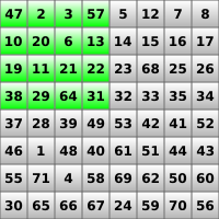
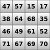
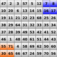
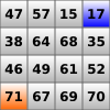
The following series of images summarizes the first reduction step of the algorithm for an 8 by 8 input texture. The image on the left shows the input texture. Highlighted in green is the range of the output texels (which are of course located in another texture). The image on the right shows the result of the first reduction pass. Observe that each texel in the output contains the local maximum of a corresponding 2 by 2 region in the input texture. This relation is further highlighted in the second row of images.

Implementation

Generic loop

In this tutorial, only the necessary steps to perform the actual reduction are explained in detail. The naming conventions are based on the Basic Math Tutorial to avoid confusion. Since the actual reduction is performed in a ping-pong manner, three different textures are required in this example: one input texture containing the input vector, and two (temporary) textures to perform the reduction itself. The following initializations are assumed:

// texture identifiers
GLuint pingpongTexID[2];
GLuint inputTexID;

// ping pong management vars
int writeTex = 0;
int readTex = 1;
GLenum attachmentpoints[] = { GL_COLOR_ATTACHMENT0_EXT, GL_COLOR_ATTACHMENT1_EXT };

All textures are assumed to be properly set up to the size sqrt(N) by sqrt(N). The texture identified by inputTexID is assumed to be already populated with the vector of length N we want to compute the maximum entry of.

The first step in the computation takes the texture identified by inputTexID as input and reduces it once into the currently writable ping-pong texture attached to an FBO. This first step is taken out of the reduction loop because we do not want to overwrite the input texture during the computation.

// enable fragment profile, bind program [...]

// enable input texture
cgGLSetTextureParameter(textureParam, inputTexID);
cgGLEnableTextureParameter(textureParam);

// set render destination
glDrawBuffer (attachmentpoints[writeTex]);

// calculate output region width and height
int outputWidth = texSize / 2;

// perform computation and ping-pong output textures
drawQuad(outputWidth,outputWidth);
swap();

Here, drawQuad(w,h) and swap() are two generic functions that draw a quad of size w by h into the output texture and swap the role of the read-only and write-only textures attached to the FBO respectively.

Next, the remaining number of reduction steps is computed and the steps are executed in a loop with the usual ping-pong technique.

// calculate number of remaining passes: log_2 of current output width
int numPasses = (int)(log((double)outputWidth)/log(2.0));

// perform remaining reduction steps
for (int i=0; i<numPasses; i++) {
  
    // input texture is read-only texture of pingpong textures
    cgGLSetTextureParameter(textureParam,pingpongTexID[readTex]);
    cgGLEnableTextureParameter(textureParam);
  
    // set render destination
    glDrawBuffer (attachmentpoints[writeTex]);

    // calculate output region width and height
    outputWidth = outputWidth / 2;

    // perform computation and ping-pong output textures
    drawQuad(outputWidth,outputWidth);
    swap();
}

In the next sections, the actual kernels used for two different ways to implement this will be discussed in detail.

Solution 1: Precomputed texcoords

Recall that we need to adjust the texture coordinates used to sample the input texture to read in 2x2 blocks. One way to do this is to pass them in using the texcoord interpolants the GL provides: With the glMultiTexCoord() routines, we can assign several sets of texture coordinates to the vertices of the rendered quad and have them automatically interpolated across the quad. So we simply pass the coordinates of the locations we want to sample in our reduction shader later on. The generic function drawQuad(w,h) is therefore adjusted as follows:

/**
 * Renders w x h quad in top left corner of the viewport.
 */
void drawQuad(int w, int h) {
    glBegin(GL_QUADS);
    glMultiTexCoord2f(GL_TEXTURE0, -0.5, -0.5);
    glMultiTexCoord2f(GL_TEXTURE1,  0.5, -0.5);
    glMultiTexCoord2f(GL_TEXTURE2, -0.5,  0.5);
    glMultiTexCoord2f(GL_TEXTURE3,  0.5,  0.5);
    glVertex2f(0.0, 0.0);

    glMultiTexCoord2f(GL_TEXTURE0, 2*w-0.5, -0.5);
    glMultiTexCoord2f(GL_TEXTURE1, 2*w+0.5, -0.5);
    glMultiTexCoord2f(GL_TEXTURE2, 2*w-0.5,  0.5);
    glMultiTexCoord2f(GL_TEXTURE3, 2*w+0.5,  0.5);
    glVertex2f(w, 0.0);

    glMultiTexCoord2f(GL_TEXTURE0, 2*w-0.5, 2*h-0.5);
    glMultiTexCoord2f(GL_TEXTURE1, 2*w+0.5, 2*h-0.5);
    glMultiTexCoord2f(GL_TEXTURE2, 2*w-0.5, 2*h+0.5);
    glMultiTexCoord2f(GL_TEXTURE3, 2*w+0.5, 2*h+0.5);
    glVertex2f(w, h);

    glMultiTexCoord2f(GL_TEXTURE0, -0.5, 2*h-0.5);
    glMultiTexCoord2f(GL_TEXTURE1,  0.5, 2*h-0.5);
    glMultiTexCoord2f(GL_TEXTURE2, -0.5, 2*h+0.5);
    glMultiTexCoord2f(GL_TEXTURE3,  0.5, 2*h+0.5);
    glVertex2f(0.0, h);
    glEnd();

}

Note that the quad covers a region of size w by h, whereas the texture coordinates cover 2w by 2h. The admittedly unfamiliar-looking modifications of the actual coordinates by plus/minus 0.5 is required to define the input coordinates for texture rectangles correctly. It is highly recommended to modify the implementation to perform just one reduction pass and print out the generated texture coordinates for a deeper insight. As texture coordinates are defined per vertex, the rasterizer will interpolate them across the quad. In the kernel, we therefore just input the interpolated coordinates and use them to sample the input texture four times. The resulting values are then fed into the max() function of Cg, and the maximum of the four values is returned.

float maximum (float2 left: TEXCOORD0,
               float2 right: TEXCOORD1,
               float2 top: TEXCOORD2,
               float2 bottom: TEXCOORD3,
               uniform samplerRECT texture) : COLOR { 
    float val1 = texRECT(texture, left);
    float val2 = texRECT(texture, right);
    float val3 = texRECT(texture, top);
    float val4 = texRECT(texture, bottom);
    return max(val1,max(val2,max(val3,val4)));
}

Note that we read in the coordinates using the register binding to the predefined TEXCOORDi identifiers, which correspond to the values we passed in per vertex using glMultiTexCoord().

A sample implementation of this solution is available for download.

Solution 2: On-the-fly texcoord manipulation

Alternatively, we can compute the offsets on-the-fly based on the output index directly in the shader. The generic function drawQuad(w,h) is in fact very simple in this approach:

void drawQuad(int w, int h) {
    glBegin(GL_QUADS);
    glVertex2f(0.0, 0.0);
    glVertex2f(w, 0.0);
    glVertex2f(w, h);
    glVertex2f(0.0, h);
    glEnd();
}

The actual computation is quite easy: First, we need to subtract 0.5 from the incoming output position to move away from the texel center to its origin. Then, we double the value and add 0.5 again to move back to the texel center. The resulting shader is:

float maximum (float2 coords: WPOS, 
               uniform samplerRECT texture) : COLOR { 
    float2 topleft = ((coords-0.5)*2.0)+0.5;
    float val1 = texRECT(texture, topleft);
    float val2 = texRECT(texture, topleft+float2(1,0));
    float val3 = texRECT(texture, topleft+float2(1,1));
    float val4 = texRECT(texture, topleft+float2(0,1));
    return max(val1,max(val2,max(val3,val4)));
}

A sample implementation of this solution is available for download. Additionally, a sample implementation using RGBA textures is provided. Except for the obvious changes regarding the texture format, the shader is modified to compute the maximum of each RGBA value into an RGBA result. The final maximum of the resulting RGBA "scalar" is calculated on the CPU. This version runs fine on ATI hardware which does not support LUMINANCE render targets as used throughout the tutorial. Please note that this modification is straight-forward on the code level and completely independent of the technique conveyed by this tutorial. Download the source file here.

Suggestions for Improvements

The implementation allows for a multitude of improvements beyond the scope of this introductory tutorial:

Instead of interpolating texture coordinates in float2 tupels, it is recommended to pair them into float4 groups, because the interpolation hardware in the rasterizer natively works on RGBA data.
The vertex shader can be used to compute the coordinates on the fly instead of calculating offsets once per fragment.
There is a certain point at which it is faster to terminate the reduction process and just compute everything in one pass or on the CPU. This needs to be benchmarked by the individual applications

Acknowledgements

I would like to thank Thomas Rohkämper for creating the images used in this tutorial. Andrew Burnett-Thompson helped with beta-testing and proofreading. Additionally, the forums at gpgpu.org always deserve proper credit.

Disclaimer and Copyright

The example code for this tutorial is released under a weakened version of the zlib/libPNG licence:

This software is provided 'as-is', without any express or implied
warranty.  In no event will the author be held liable for any 
damages arising from the use of this software. 

Permission is granted to anyone to use this software for any 
purpose, including commercial applications, and to alter it 
and redistribute it freely.

Feedback (preferably by e-mail) is appreciated!

Dominik Göddeke -- GPGPU::Reduction Tutorial