The optimization codes were compiled with the f77 compiler using the
-O3 (aggressive code optimization) compilation flag on a
Silicon Graphics Power Indigo![]() with Mips R8000 chip, 192 MB main memory
and IRIX 6.0.1 operating system. The machine precision on this machine is
approximately
with Mips R8000 chip, 192 MB main memory
and IRIX 6.0.1 operating system. The machine precision on this machine is
approximately ![]() . All facility distributions were computed
on this machine. The computation times were obtained by the
IRIX time command.
. All facility distributions were computed
on this machine. The computation times were obtained by the
IRIX time command.
We computed facility distributions for problems with N facilities,
![]() ,
, ![]() , and, additionally,
, and, additionally, ![]() .
The last set of distributions was computed for benchmarking reasons.
The biggest problem solved had therefore N = 1600 facilities,
which resulted in a nonlinear nonconvex global optimization problem with
3197 unknowns and 6394 constraints.
.
The last set of distributions was computed for benchmarking reasons.
The biggest problem solved had therefore N = 1600 facilities,
which resulted in a nonlinear nonconvex global optimization problem with
3197 unknowns and 6394 constraints.
Figure 1 shows the computation time for the first (simulated annealing, SA) and the second (limited-memory BFGS, L-BFGS) phase in Stage 1. A detailed table of all computation times can be found in the appendix, see Table 2. As it can be seen, the bottle neck of the computation is the first part of the optimization process, i. e. obtaining a point distribution which is not too bad. Note that only one run of the simulated annealing algorithm in Phase I was needed to produce a good starting distribution for Phase II. The biggest problem took 722 minutes (about 12 hours) computation time in Phase I, followed by another 79 minutes for Phase II.
=85mm
time1.ps
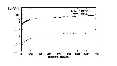
Figure ![]()
![]() for the distribution calculated by the simulated annealing algorithm. The
L-BFGS algorithm then refined this number to
for the distribution calculated by the simulated annealing algorithm. The
L-BFGS algorithm then refined this number to
![]() .
Detailed results can be found in Table 3 in the appendix.
.
Detailed results can be found in Table 3 in the appendix.
 Figure
 ![]()
Figure ![]()
Figure ![]()
Figure ![]()
Figure ![]()
![]() ,
, ![]() , but their
algorithm nevertheless produced completely different facility distributions.
, but their
algorithm nevertheless produced completely different facility distributions.