Numerical tests

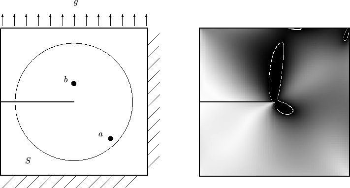
We have applied our technique for a posteriori error estimation to a proto-typical test problem in plasticity which has already been considered in [31] in the context of linear elasticity. Another application to a benchmark problem in perfect plasticity will be presented in [33]. Our test case is the plane strain model of a square elastic disc with a crack subjected to a growing (constant) boundary traction acting along the upper boundary (see Figure 3). Along the right-hand side and the lower boundary the body is fixed and the remaining part of the boundary (including the crack) is left free. This problem is interesting as its solution develops a singularity at the tip of the crack where in the elastic case a stress concentration occurs with an asymptotic behaviour (expressed in terms of polar coordinates) of the form  $\sigma$ $\approx$ r^-1/2 . Hence, local plastification will occur right form the beginning of the loading process.

We consider the case of the linear isotropic material law in the form

$$\sigma \mu \epsilon \kappa$$

and the perfect plastic behaviour is determined by the flow function

$$\cal {F} \sigma \sigma^{D}_{} \sqrt{\tfrac{2}{3}} \sigma_{0}^{} \le$$

The values for the above parameters are set to

$$\kappa \mu \sigma_{0}^{}$$

which corresponds to the properties of Aluminum (cf. [13]). The boundary traction is assumed in the form  g = tg₀ , with  g₀ = 100  and  t > 0 . In the case of the Hencky model, we take  t_lim = 2.234 , since already for  t = 2.3 , plastic collapse occurs.

Abbildung: Geometry of the square disc test problem and plot of  |$\sigma^{D}_{}$|  (plastic regions black) computed on a mesh with  N $\approx$ 64, 000  cells

From the engineering point of view it is most interesting to know the corresponding stress intensity factor which can be expressed in terms of the (unknown) displacement  u  by evaluating contour integrals of the form (see [15] and the literature cited therein)

$$\int_{S}^{} \psi \sigma \int_{S}^{} \sigma \psi$$ (50)

where S is a suitable circular path around the tip of the crack, and $\psi$($\theta$) are certain trigonometric polynomials. These integrals are usually generated numerically from a computed solution u_h . The question is now, what is the most economical mesh to compute J_u(u) and J_$\sigma$(u) to best accuracy. The traditional answer, based on a priori error analysis, is that one should use a mesh which is optimal for the energy error. This requires a graded refinement towards the corner point of the form  h(r) $\approx$ rh . However, this asymptotic information does not provide a useful error bound on the meshes actually used. A further complication arises from the weak stress singularity occurring at the point of discontinuity of the boundary condition at the upper right corner. In such a situation when several accuracy limiting effects occur simultaneously mere asymptotic error analysis will hardly lead to reliable error bounds. Here, our new approach offers the possibility of rigorous error control. In order to demonstrate the local features of this technique, we also consider the computation of the stress point-value  $\sigma_{11}^{}$(a)  (see Figure 3).

Finally, we apply the nonstationary Prandtl-Reuss model for the computation of the stress point-value  $\sigma_{11}^{}$(b)  (see Figure 3). This demonstrates that, at least on a heuristic basis, our approach also works within a incremental loading process. Further applications based on the Prandtl-Reuss model will be presented in [34].

The solutions on very fine (adaptive) meshes with about 200,000 cells are taken as reference solutions  u_ref  for determining the relative errors

E^rel  : =  | J(u_h) - J(u_ref)|/| J(u_ref)|

on coarser meshes, while

Ratio  : =  $${\frac{\eta(u_h)}{\vert J(u_{ref})-J(u_h)\vert}}$$

are the overestimation factors of the different error estimators. For mesh refinement (and coarsening) we use the strategy described above.