


Nächste Seite: Mesh refinement strategy
Aufwärts: The new adaptive finite
Vorherige Seite: The new adaptive finite
Now, we will consider a posteriori error estimates for the discretization
process described above, i.e., for the error in the displacement, u - uh , and
for the error in the corresponding stresses,
 -
-  . We begin with two of
the traditional strategies for error estimation.
. We begin with two of
the traditional strategies for error estimation.
1) The ZZ-approach:
The error indicator proposed by Zienkiewicz and Zhu [22] for finite
element models in structural mechanics is based on the idea of higher-order
stress recovery by local averaging. The element-wise error
| - |K is thought to be well represented by the auxiliar quantity
 : = |
: = | h - |K , where
h is a local
(super-convergent) approximation of
. The corresponding (heuristic) global
error estimator reads
h - |K , where
h is a local
(super-convergent) approximation of
. The corresponding (heuristic) global
error estimator reads
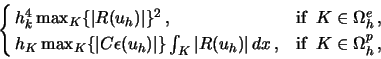
| - -  | |   : = : =   | | h - |K2 h - |K2 . . |
(47) |
For our purpose we assume the discrete stresses to be constant over each cell.
One possible construction of
h is the patch-wise L2-projection
PK onto the space of (bi-)linear shape functions. Here the nodal value
at a point of the triangulation determining
h is obtained by
averaging the cell-wise constant values of of those cells having this
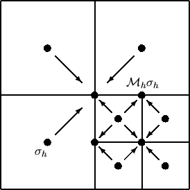
point in common. For cells containing hanging nodes this process is appopriately
modified (see Figure 2).
Abbildung 2:
Sketch: Averaging process for ZZ-Indicator
 |
2) An energy error estimator:
Johnson and Hansbo [11] proposed an error estimator for the primal-mixed
formulation of the Hencky model which is based on monotinicity properties of the
energy form and, under some additional heuristic assumptions, bounds the error in
the global energy norm. Let
 and
and
 denote the union of elements where the discrete solution behaves elastic and plastic,
respectively. Then, the estimator reads
denote the union of elements where the discrete solution behaves elastic and plastic,
respectively. Then, the estimator reads
with the local error indicators
 : = : =  |
|
where on each element
K 
 h the local residual is defined by
R(
uh) : = |
divC
(
uh)| +
 hK-1
hK-1|[
n . C(
uh)]| .
Here, Ci is some interpolation constant usually set to one.
This estimator is rather heuristic, as it relies on the assumption that the
plastification zone is already correctly captured on the current mesh. Furthermore,
it is of only sub-optimal order in the plastic zone which results in mesh over-refinement
in  , though the stresses are suspected to be rather smooth there.
The ZZ-estimator
(39) does not suffer from this deficiency as it essentially
relies on the smoothness of . Hence, we are led to modify the estimator
(40) by replacing the obviously too crude a bound
maxK| C
, though the stresses are suspected to be rather smooth there.
The ZZ-estimator
(39) does not suffer from this deficiency as it essentially
relies on the smoothness of . Hence, we are led to modify the estimator
(40) by replacing the obviously too crude a bound
maxK| C (uh)| in the plastic zone by
maxK| C(uh) - hC(uh)| .
This gives us the local (still heuristic) error indicators
(uh)| in the plastic zone by
maxK| C(uh) - hC(uh)| .
This gives us the local (still heuristic) error indicators
: = 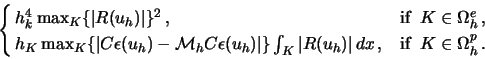 |
|
3) The weighted local error estimator:
Finally, we recall our weighted a posteriori error estimator for the primal
formulation (27) of the Hencky problem,
with the local residuals
 : = hK| f - divC( : = hK| f - divC( uh)|K + hK1/2| n . [C(uh)]| uh)|K + hK1/2| n . [C(uh)]| K , K , |
|
and the weights
obtained from the approximate dual solution
 .
.
Nächste Seite: Mesh refinement strategy
Aufwärts: The new adaptive finite
Vorherige Seite: The new adaptive finite
sutti
2000-04-19