DFG flow around cylinder benchmark 2D-2, time-periodic case (Re=100)
This benchmark simulates the time-periodic behaviour of a fluid in a pipe with a circular obstacle. It is set up in 2D with geometry data similar to the Re=20 case.
Geometry and flow configuration
The underlying geometry is a pipe without a circular cylinder $\Omega=[0,2.2] \times [0,0.41] \setminus B_r(0.2,0.2)$ with $r=0.05$. Taking a fluid density of $\rho=1.0$, the fluid is characterised by the nonstationary Navier-Stokes equations
$$ u_t - \nu\Delta u + u\nabla u + \nabla p = 0,\qquad \text{\div }u = 0 $$
with $u$ defining the velocity and $p$ the pressure. The kinematic viscosity is taken as
$$ \nu = 0.001. $$

Boundary conditions
For the lower and upper walls $\Gamma_1=[0,2.2] \times {0}$ and $\Gamma_1=[0,2.2] \times {0.41}$ as well as the boundary $S=\partial B_r(0.2,0.2)$, no-slip boundary conditions are defined,
$$ u_{|\Gamma_1} = u_{|\Gamma_3} = u_{|S} = 0. $$
On the left edge $\Gamma_4={0} \times [0,0.41]$, a parabolic inflow profile is prescribed,
$$ u(0,y) = \left( \frac{4 U y (0.41-y)}{0.41^2} , 0 \right), $$
with a maximum velocity $U=1.5$. On the right edge $\Gamma_4={2.2}\times[0,0.41]$, do-nothing boundary conditions define the outflow,
$$ \nu \partial_\eta u - p \eta = 0 $$
with $\eta$ denoting the outer normal vector.
Reynolds number
For a maximum velocity of $U=1.5$, the parabolic profile results in a mean velocity
$$ U_\text{mean} = \frac{2}{3}\cdot 1.5 = 1.0. $$
The characteristic length of the flow configuration is
$$ L = 2\cdot 0.05 = 0.1 $$
the diameter of the object perpendicular to the flow direction. This results in a Reynolds number
$$ \text{Re} = \frac{U_\text{mean} L}{\nu} = \frac{1.0 \cdot 0.1}{0.001} = 100. $$
For this Reynolds number, the flow turns into a time-periodic behaviour with a vortex shedding behind the cylinder. This is visualised in the Figure below.

Velocity magnitude

Velocity magnitude with SurfaceLIC representation visualising the streamlines

Pressure
Important numerical quantities
For the numerical comparison of data, the forces around the circle are measured. These drag and lift forces are defined by
$$ \begin{pmatrix} F_D F_L \end{pmatrix} = \int_{S} \sigma \eta ds $$
with $\eta$ denoting the outer normal vector of the circle. The stress tensor $\sigma$ in this formula is defined as
$$ \sigma := \nu \nabla u - p I. $$
A not so straightforward calculation which exploits $u_{|S}=0$ can be used to derive the following formulas for the drag and lift force, which can alternatively be used in 2D, see [2]:
$$ F_D = \int_S \left(\nu \frac{\partial u_{\tau}}{\partial_\eta} \eta_2 - p \eta_1 \right) ds,\quad F_L = - \int_S \left(\nu \frac{\partial u_{\tau}}{\partial_\eta} \eta_1 + p \eta_2 \right) ds $$
From the forces, one obtains the dimensionless drag and lift coefficients,
$$ C_D = \frac{2}{U_\text{mean}^2 L} F_D,\qquad C_L = \frac{2}{U_\text{mean}^2 L} F_L. $$
Setup of the test and data measurement
To measure numerical data, one needs a fully developed time-periodic solution. This can be achieved, e.g., using the following procedure:
- Start with a zero solution and simulate about 3.5 seconds simulation time with a coarse time step to calculate an initial solution.
- Simulate about 25 seconds simulation time with a finer time step; the flow should be fully developed at that time.
- Between 25 and 30 seconds of simulation time, take an arbitrary cycle of the nonstationary flow for comparison.
- A cycle starts at a time instant $t_0$ where the lift coefficient $C_L$ is smallest and ends at a time instant $t_1 = t_0 + 1/f$ when $C_L$ is smallest again. $f$ defines the frequency and $1/f$ the length of the cycle, which should be about 1/f=0.33 seconds simulation time.
The following numerical quantities are measured:
- The drag and lift coefficients $C_D$ and $C_L$ over the time interval $[t_0,t_1]$.
- the pressure difference $p_\text{diff}:=p(a_1)-p(a_2)$ in the points $a_1=(0.15,0.2)$ and $a_2=(0.25,0.2)$ on the front and rear side of the cylinder over the time interval $[t_0,t_1]$,
- the Strouhal number $$\text{St} = \frac{L f}{U_\text{mean}},$$
- $\min(C_D)$, $\max(C_D)$, $\text{mean}(C_D)$, $\text{amp}(C_D)$ in the time interval $[t_0,t_1]$,
- $\min(C_L)$, $\max(C_L)$, $\text{mean}(C_L)$, $\text{amp}(C_L)$ in the time interval $[t_0,t_1]$,
with the amplitude amp=max-min and the mean value mean=(max+min)/2.
Test configuration
The test configuration used to generate the reference tests reads as follows:
- Finite element discretisation with $Q_2/P_1^\text{disc}$ in space. No stabilisation.
- Crank-Nicolson time discretisation scheme.
- Time step: $k=1/100$, $1/200$ and $1/400$.
- Regular refinement of the mesh shown below. For different refinement refinement levels, the following table shows the number of elements and degrees of freedom in the underlying system:
| Level | #Vertices | #Elements | #degrees of freedom |
|---|---|---|---|
| 1 | 156 | 130 | 702 |
| 2 | 572 | 520 | 2704 |
| 3 | 2184 | 2080 | 10608 |
| 4 | 8528 | 8320 | 42016 |
| 5 | 33696 | 33280 | 167232 |
| 6 | 133952 | 133120 | 667264 |

Exemplary Results
The first table shows information about min/max drag coefficient values:
| Lv. | k | $\min(C_D)$ | $\max(C_D)$ | mean$(C_D)$ | amp$(C_D)$ |
|---|---|---|---|---|---|
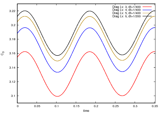
| 3 | 1/100 | 3.0997 | 3.1626 | 3.1311 | 6.292E-02 |
| 3 | 1/200 | 3.0993 | 3.1625 | 3.1309 | 6.312E-02 |
| 3 | 1/400 | 3.0992 | 3.1624 | 3.1308 | 6.315E-02 |
| 4 | 1/100 | 3.1338 | 3.1964 | 3.1651 | 6.252E-02 |
| 4 | 1/200 | 3.1333 | 3.1962 | 3.1647 | 6.283E-02 |
| 4 | 1/400 | 3.1333 | 3.1958 | 3.1645 | 6.249E-02 |
| 5 | 1/100 | 3.1497 | 3.2124 | 3.1811 | 6.269E-02 |
| 5 | 1/200 | 3.1494 | 3.2122 | 3.1808 | 6.287E-02 |
| 5 | 1/400 | 3.1493 | 3.2122 | 3.1807 | 6.292E-02 |
| 6 | 1/200 | 3.1569 | 3.2200 | 3.1884 | 6.310E-02 |
The second table shows information about min/max lift coefficient values:
| Lv. | k | $\min(C_L)$ | $\max(C_L)$ | mean$(C_L)$ | amp$(C_L)$ |
|---|---|---|---|---|---|
| 3 | 1/100 | -1.0112 | 0.9805 | -0.0154 | 1.992E+00 |
| 3 | 1/200 | -1.0159 | 0.9810 | -0.0174 | 1.997E+00 |
| 3 | 1/400 | -1.0155 | 0.9805 | -0.0175 | 1.996E+00 |
| 4 | 1/100 | -1.0155 | 0.9838 | -0.0158 | 1.999E+00 |
| 4 | 1/200 | -1.0182 | 0.9838 | -0.0172 | 2.002E+00 |
| 4 | 1/400 | -1.0181 | 0.9835 | -0.0173 | 2.002E+00 |
| 5 | 1/100 | -1.0169 | 0.9859 | -0.0155 | 2.003E+00 |
| 5 | 1/200 | -1.0211 | 0.9818 | -0.0196 | 2.003E+00 |
| 5 | 1/400 | -1.0206 | 0.9860 | -0.0173 | 2.007E+00 |
| 6 | 1/200 | -1.0206 | 0.9859 | -0.0173 | 2.008E+00 |
The third table shows the length of the cycle and the Strouhal number.
| Lv. | k | 1/f | St |
|---|---|---|---|
| 3 | 1/100 | 3.3000E-01 | 0.30303 |
| 3 | 1/200 | 3.3000E-01 | 0.30303 |
| 3 | 1/400 | 3.3000E-01 | 0.30303 |
| 4 | 1/100 | 3.4000E-01 | 0.29411 |
| 4 | 1/200 | 3.3000E-01 | 0.30303 |
| 4 | 1/400 | 3.3250E-01 | 0.30075 |
| 5 | 1/100 | 3.3000E-01 | 0.30303 |
| 5 | 1/200 | 3.3000E-01 | 0.30303 |
| 5 | 1/400 | 3.3000E-01 | 0.30303 |
| 6 | 1/200 | 3.3125E-01 | 0.30188 |
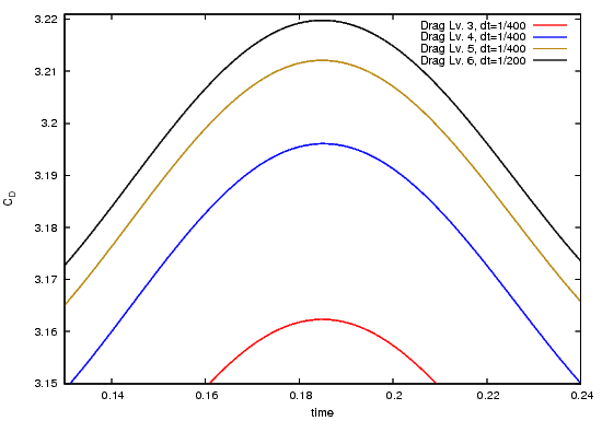
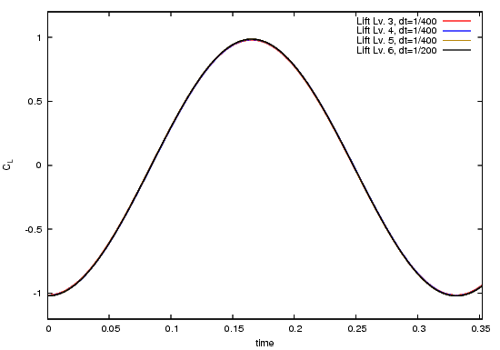
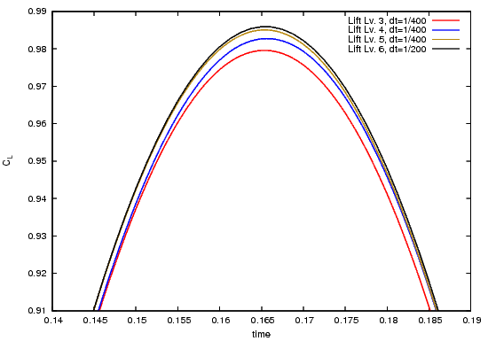
In the following, a couple of pictures highlight the numerical solutions. Due to the fact, that the cycle always started at different $t_0$ depending on the underlying discretisations, the curves are shifted in time such that $t_0$ matched.
The following pictures shows the drag coefficient over time, once over the complete time interval $[t_0,t_1]$, once near the maximum value:


The following pictures shows the lift coefficient over time, once over the complete time interval $[t_0,t_1]$, once near the maximum value:


The following pictures shows the pressure difference $p_\text{diff}$ over the complete time interval $[t_0,t_1]$:

Reference results
From the following table, the underlying GNUPLOT data can be downloaded. The files provide the data for different discretisations, different refinement levels in space and different refinement levels in time.
| Description | File |
|---|---|
| Drag/Lift, $\tilde Q_1/Q_0$ | draglift_q1t_cn_lv3-6_dt1-4.zip |
| Drag/Lift, $Q_2/P_1^\text{disc}$ | draglift_q2_cn_lv3-6_dt1-4.zip |
| Pressure, $\tilde Q_1/Q_0$ | pressure_q1t_cn_lv3-6_dt1-4.zip |
| Pressure, $Q_2/P_1^\text{disc}$ | pressure_q2_cn_lv3-6_dt1-4.zip |
| GNUplot command file for $Q_2$ plots | plot_bench2.plt |
New reference results
The following results were computed using a higher-order line integration scheme for the drag/lift computation around the circle. The results are therefore of higher quality compared to the results above. A discussion with corresponding pictures will be added to this page soon, replacing the old results.
| Description | File |
|---|---|
| Drag/Lift/Pressure/y-velocity and GNUPlot file, $Q_2/P_1^\text{disc}$ | 20141124_dfg_bench2_official.zip |
References
| Id | Title |
|---|---|
| [1] | Turek, Schaefer; Benchmark computations of laminar flow around cylinder; in Flow Simulation with High-Performance Computers II, Notes on Numerical Fluid Mechanics 52, 547-566, Vieweg 1996 |
| [2] | John; Higher order Finite element methods and multigrid solvers in a benchmark problem for the 3D Navier-Stokes equations; Int. J. Numer. Meth. Fluids 2002; 40: 775-798 (DOI: 10.1002/ d.377) |
